In this blog post, we are going to perform a simple version of the spectral clustering algorithm for clustering the data points.

Clustering is a type of machine learning task, and it helps people to cluster their data points into different groups.

Today, we are going to introduce an clustering algorithm call Spectral Clustering. Before we dive into the spectral clustering, we first try an clustering example using K-means algorithm.

# Import required packages
import numpy as np
from sklearn import datasets
from matplotlib import pyplot as plt

K-means algorithm is a very common method in clustering, and it cluster the data points into K clusters in which each observation belongs to the cluster with the nearest mean. This algorithm usually work well in most cases.

Now, let’s first generate a fake dataset using make_blobs() method that we’ve imported from ‘datasets’ module in ‘sklearn’ package.

n = 200
np.random.seed(1111)
X, y = datasets.make_blobs(n_samples=n, shuffle=True, random_state=None, centers = 2, cluster_std = 2.0)
plt.scatter(X[:,0], X[:,1])

<matplotlib.collections.PathCollection at 0x7f7a62923ee0>

# Perform K-means clustering
from sklearn.cluster import KMeans
km = KMeans(n_clusters = 2)
km.fit(X)

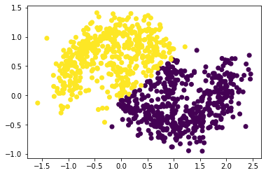
plt.scatter(X[:,0], X[:,1], c = km.predict(X))

<matplotlib.collections.PathCollection at 0x7f7a80665c10>

Harder Clustering

However, if our data points are “shaped weird”, k-means clustering may not work well. In the example below, we are going to create another dataset example using make_moons() function.

np.random.seed(1234)
n = 200
X, y = datasets.make_moons(n_samples=n, shuffle=True, noise=0.05, random_state=None)
plt.scatter(X[:,0], X[:,1])

<matplotlib.collections.PathCollection at 0x7f7a7083d4c0>

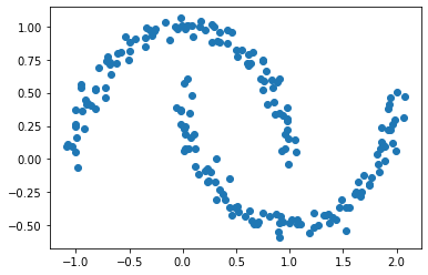
For this plot, we can still make out two meaningful clusters in the data. However, k-means won’t work well here.

km = KMeans(n_clusters = 2)
km.fit(X)
plt.scatter(X[:,0], X[:,1], c = km.predict(X))

<matplotlib.collections.PathCollection at 0x7f7a806f82b0>

As we can see, the clustering result using k-mean is not correct!! Today, we are going to introduce spectral clustering, and this algorithm will work well for above data points.

Part A - Similarity Matrix

The first thing we are going to do is to construct the similarity matrix \(\mathbf{A}\). \(\mathbf{A}\) should be a matrix (2d np.ndarray) with shape (n, n) .

We will use a parameter epsilon. Entry A[i,j] should be equal to 1 if X[i] (the coordinates of data point i) is within distance epsilon of X[j] (the coordinates of data point j), and 0 otherwise.

The diagonal entries A[i,i] should all be equal to zero. function np.fill_diagonal() is a good way to help us achieve this.

For this part, we use epsilon = 0.4.

epsilon = 0.4

# Check the shape of X
X.shape

(200, 2)

from sklearn.metrics.pairwise import pairwise_distances
# Construct the similarity matrix A
# Function that compute all the pairwise distance
A = pairwise_distances(X, X)
# Check the shape of matrix A
A.shape

(200, 200)

Let’s take a look at our similarity matrix A.

A[:5, :5]

array([[0.        , 1.27292462, 1.33315598, 1.97506495, 2.43337261],
       [1.27292462, 0.        , 1.46325112, 1.93152405, 2.18793876],
       [1.33315598, 1.46325112, 0.        , 0.64238147, 1.10996726],
       [1.97506495, 1.93152405, 0.64238147, 0.        , 0.50493603],
       [2.43337261, 2.18793876, 1.10996726, 0.50493603, 0.        ]])

The matrix A now stores the pairwise distances rather than 0 and 1. We are going to replace all elements that are less than eplison with 1 and other elements with 0. In this case, we will use np.where() method to achieve this.

# Let A[i, j] = 1 if X[i] is within distance epsilon of X[j]
# Otherwise, A[i, j] = 0
A = np.where(A < epsilon, 1, 0)

# The diagonal entries should be all zero
np.fill_diagonal(A, 0)

Let’s take a look at matrix A.

# Check the matrix A
A[:5, :5]

array([[0, 0, 0, 0, 0],
       [0, 0, 0, 0, 0],
       [0, 0, 0, 0, 0],
       [0, 0, 0, 0, 0],
       [0, 0, 0, 0, 0]])

Part B

Our similarity matrix A from Part A now contains information about which points are near (within distance epsilon) which other points. We will now partition the rows and columns of A.

Let \(d_i = \sum_{j = 1}^n a_{ij}\) be the \(i\)th row-sum of \(\mathbf{A}\), which is also called the degree of \(i\). Let \(C_0\) and \(C_1\) be two clusters of the data points. We assume that every data point is in either \(C_0\) or \(C_1\). The cluster membership as being specified by y. We think of y[i] as being the label of point i. So, if y[i] = 1, then point i (and therefore row \(i\) of \(\mathbf{A}\)) is an element of cluster \(C_1\).

The binary norm cut objective of a matrix \(\mathbf{A}\) is the function

In this expression,

• \(\mathbf{cut}(C_0, C_1) \equiv \sum_{i \in C_0, j \in C_1} a_{ij}\) is the cut of the clusters \(C_0\) and \(C_1\).
• \(\mathbf{vol}(C_0) \equiv \sum_{i \in C_0}d_i\), where \(d_i = \sum_{j = 1}^n a_{ij}\) is the degree of row \(i\) (the total number of all other rows related to row \(i\) through \(A\)). The volume of cluster \(C_0\) is a measure of the size of the cluster.

A pair of clusters \(C_0\) and \(C_1\) is considered to be a “good” partition of the data when \(N_{\mathbf{A}}(C_0, C_1)\) is small. To see why, let’s look at each of the two factors in this objective function separately.

B.1 The Cut Term

First, the cut term \(\mathbf{cut}(C_0, C_1)\) is the number of nonzero entries in \(\mathbf{A}\) that relate points in cluster \(C_0\) to points in cluster \(C_1\). Saying that this term should be small is the same as saying that points in \(C_0\) shouldn’t usually be very close to points in \(C_1\).

You will then write a function called cut(A,y) to compute the cut term. You can compute it by summing up the entries A[i,j] for each pair of points (i,j) in different clusters.

There is a solution for computing the cut term that uses only numpy tools and no loops. However, it’s fine to use for-loops for this part only – we’re going to see a more efficient approach later.

def cut(A, y):
    '''
    This function compute the cut 
    term by summing up the entries A[i,j]
    for each pair of data points in different
    clusters.
    
    Parameters:
     - A : The similarity matrix
             (2d numpy array)
     - y : The lables of data points
             (1d numpy array)
    '''
    sum = 0
    for i in range(n):
        for j in range(n):
            if y[i] == 0 and y[j] == 1:
                sum += A[i][j]
    return sum

Now, we will use the above cut() function to compute the cut objective for the true cluster y.

cut(A, y)

13

Next, we will generate a random vector of random labels of length n, with each label equal to either 0 or 1. If we check the cut term for the random labels, we should be able to find that the cut objective for the true labels is much smaller than the cut objective for the random labels.

# Creating random labels of size n, with either 0, 1
random_labels = np.random.randint(2, size = n)

# check the cut
cut(A, random_labels)

1150

If we get the above result, we will be able to see that the cut objective for these random labels are larger than for the true labels.

B.2 The Volume Term

Now take a look at the second factor in the norm cut objective. This is the volume term. As mentioned above, the volume of cluster \(C_0\) is a measure of how “big” cluster \(C_0\) is. If we choose cluster \(C_0\) to be small, then \(\mathbf{vol}(C_0)\) will be small and \(\frac{1}{\mathbf{vol}(C_0)}\) will be large, leading to an undesirable higher objective value.

Synthesizing, the binary normcut objective asks us to find clusters \(C_0\) and \(C_1\) such that:

1. There are relatively few entries of \(\mathbf{A}\) that join \(C_0\) and \(C_1\).
2. Neither \(C_0\) and \(C_1\) are too small.

Write a function called vols(A,y) which computes the volumes of \(C_0\) and \(C_1\), returning them as a tuple. For example, v0, v1 = vols(A,y) should result in v0 holding the volume of cluster 0 and v1 holding the volume of cluster 1. Then, write a function called normcut(A,y) which uses cut(A,y) and vols(A,y) to compute the binary normalized cut objective of a matrix A with clustering vector y.

Note: No for-loops in this part. Each of these functions should be implemented in five lines or less.

def vols(A, y):
    # volume of cluster C0
    v0 = A[y == 0].sum()
    
    # volumn of cluster C1
    v1 = A[y == 1].sum()
    
    return (v0, v1)

def normcut(A, y):
    # Extract volumes of C0 and C1
    v0, v1 = vols(A, y)
    
    # Compute the binary norm cut
    # objective of th matrix
    norm = cut(A, y)*((1/v0) + (1/v1))
    
    return norm

Now, compare the normcut objective using both the true labels y and the fake labels you generated above. What do you observe about the normcut for the true labels when compared to the normcut for the fake labels?

normcut(A, y)

0.011518412331615225

normcut(A, random_labels)

1.0240023597759158

By observing the above results, we can see that the normcut for the true labels compared to normcut for false labels are much smaller.

Part C

We have now defined a normalized cut objective which takes small values when the input clusters are (a) joined by relatively few entries in \(A\) and (b) not too small. One approach to clustering is to try to find a cluster vector y such that normcut(A,y) is small. However, this is an NP-hard combinatorial optimization problem, which means that may not be possible to find the best clustering in practical time, even for relatively small data sets. We need a math trick!

Here’s the trick: define a new vector \(\mathbf{z} \in \mathbb{R}^n\) such that:

Note that the signs of the elements of \(\mathbf{z}\) contain all the information from \(\mathbf{y}\): if \(i\) is in cluster \(C_0\), then \(y_i = 0\) and \(z_i > 0\).

Next, if you like linear algebra, you can show that

where \(\mathbf{D}\) is the diagonal matrix with nonzero entries \(d_{ii} = d_i\), and where \(d_i = \sum_{j = 1}^n a_i\) is the degree (row-sum) from before.

Programming Note

You can compute \(\mathbf{z}^T\mathbf{D}\mathbf{z}\) as z@D@z, provided that you have constructed these objects correctly.

Note

np.isclose(a,b) is a good way to check if a is “close” to b, in the sense that they differ by less than the smallest amount that the computer is (by default) able to quantify.

Also, still no for-loops.

First of all, let’s write a function called transform(A,y) to compute the appropriate \(\mathbf{z}\) vector given A and y, using the formula above.

def transform(A, y):
    v0, v1 = vols(A, y)
    z = np.where(y == 0, 1/v0, -1/v1)
    return z

Secondly, We are going to check the equation above that relates the matrix product to the normcut objective, by computing each side separately and checking that they are equal.

Then, we should also check the identity \(\mathbf{z}^T\mathbf{D}\mathbb{1} = 0\), where \(\mathbb{1}\) is the vector of n ones (i.e. np.ones(n)). This identity effectively says that \(\mathbf{z}\) should contain roughly as many positive as negative entries.

# left hand side
LHS = normcut(A, y)

# diagonal matrix
D = np.diag(A.sum(axis = 0))

# Compute Z
z = transform(A, y)

# Compute the Right hand side
RHS = (z@(D-A)@z) / (z@D@z)

Finally, let’s check if a is “close” to b by using np.isclose() function.

# check if a is "close" to b
np.isclose(LHS, RHS)

True

Part D

From part C, we see that minimizing the normcut objective is related to the problem of minimizing the function

subject to the condition \(\mathbf{z}^T\mathbf{D}\mathbb{1} = 0\).

It’s actually possible to incorporate the above condition into the optimization task by substituting for \(\mathbf{z}\) the orthogonal complement of \(\mathbf{z}\) relative to \(\mathbf{D}\mathbf{1}\).

In the code below, we define function orth() and orth_obj() to handle this.

def orth(u, v):
    return (u @ v) / (v @ v) * v

e = np.ones(n) 

d = D @ e

def orth_obj(z):
    z_o = z - orth(z, d)
    return (z_o @ (D - A) @ z_o)/(z_o @ D @ z_o)

We can use the minimize function from scipy.optimize module to minimize the function orth_obj with respect to \(\mathbf{z}\).

In part C, we originally specified that each entries of z should be either 0 or 1. However, now we are allowing the entries to take any value. Thus, we are no longer optimizing the normcut objective exactly. This is the continuous relaxation of the normcut problem.

import scipy.optimize
z_min = scipy.optimize.minimize(orth_obj, np.ones(len(z))).x

The method above might take a little while. Don’t worry about that!

Part E

Recall that, by design, only the sign of z_min[i] actually contains information about the cluster label of data point i. Plot the original data, using one color for points such that z_min[i] < 0 and another color for points such that z_min[i] >= 0.

# If z_min[i] < 0, label 1
# otherwise, label 0
labels = np.where(z_min < 0, 1, 0)

# plot the data points
plt.scatter(X[:, 0], X[:, 1], c = labels)

<matplotlib.collections.PathCollection at 0x7f7a62d1aaf0>

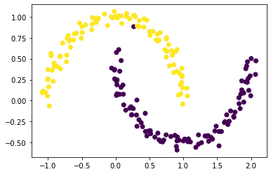
By looking at the above scatter plot, we see that we are able to cluster these data points well!

Part F

Explicitly optimizing the orthogonal objective is way too slow to be practical. If spectral clustering required that we do this each time, no one would use it.

The reason that spectral clustering actually matters, and indeed the reason that spectral clustering is called spectral clustering, is that we can actually solve the problem from Part E using eigenvalues and eigenvectors of matrices.

Recall that what we would like to do is minimize the function

with respect to \(\mathbf{z}$, subject to the condition $\mathbf{z}^T\mathbf{D}\mathbb{1} = 0\).

The Rayleigh-Ritz Theorem states that the minimizing \(\mathbf{z}\) must be the solution with smallest eigenvalue of the generalized eigenvalue problem

which is equivalent to the standard eigenvalue problem

Why is this helpful? Well, \(\mathbb{1}\) is actually the eigenvector with smallest eigenvalue of the matrix \(\mathbf{D}^{-1}(\mathbf{D} - \mathbf{A})\).

So, the vector \(\mathbf{z}\) that we want must be the eigenvector with the second-smallest eigenvalue.

Construct the matrix \(\mathbf{L} = \mathbf{D}^{-1}(\mathbf{D} - \mathbf{A})\), which is often called the (normalized) Laplacian matrix of the similarity matrix \(\mathbf{A}\). Find the eigenvector corresponding to its second-smallest eigenvalue, and call it z_eig. Then, plot the data again, using the sign of z_eig as the color. How did we do?

# Constructing the (normalized) Laplacian matrix
L = np.linalg.inv(D)@(D-A)

# Extract the eigenvalues and eigenvector
eigenvalue, eigenvector = np.linalg.eig(L)

# Sorted the eigenvector corresponding to
# the second smallest eigenvalue
sorted_eigenvector = eigenvector[:, np.argsort(eigenvalue)]

# Extract our second smallest eigenvector
z_eig = sorted_eigenvector[:, 1]

# Plot the data again using z_eig as the color
labels_2 = np.where(z_eig < 0, 1, 0)
plt.scatter(X[:, 0], X[:, 1], c = labels_2)

<matplotlib.collections.PathCollection at 0x7f7a706273a0>

From the plot above, we can see that the data are clustered well! Besides, it was much faster perform the clustering.

Part G

Synthesize your results from the previous parts. In particular, write a function called spectral_clustering(X, epsilon) which takes in the input data X (in the same format as Part A) and the distance threshold epsilon and performs spectral clustering, returning an array of binary labels indicating whether data point i is in group 0 or group 1. Demonstrate your function using the supplied data from the beginning of the problem.

Outline

Given data, we should follow the guideline below:

1. Construct the similarity matrix.
2. Construct the Laplacian matrix.
3. Compute the eigenvector with second-smallest eigenvalue of the Laplacian matrix.
4. Return labels based on this eigenvector.

def spectral_clustering(X, epsilon):
    '''
    This function perform spectral clustering
    method to cluster the data points.
    
    Parameters:
        - X : The input data points
                (numpy array)
        - epsilon: The distance threshold
                (float)
    Return:
        - labels: an array of binary labels
        indicating whether the data point should
        be in group 0 or group 1.
    '''
    ## 1. Construct the similarity matrix
    A = pairwise_distances(X, X)
    # Let A[i, j] = 1 if X[i] is within distance epsilon of X[j]
    # Otherwise, A[i, j] = 0
    A = np.where(A < epsilon, 1, 0)
    # The diagonal entries should be all zero
    np.fill_diagonal(A, 0)
    
    ## 2. Construct the Laplacian matrix
    D = np.diag(A.sum(axis = 0))
    L = np.linalg.inv(D)@(D-A)
    
    ## 3. Compute the eigenvector with second-
    ##    smallest eigenvalue of the Laplacian matrix
    eigenvalue, eigenvector = np.linalg.eig(L)
    sorted_eigenvector = eigenvector[:, np.argsort(eigenvalue)]
    z_eig = sorted_eigenvector[:, 1]
    
    ## 4. Return labels based on z_eig - eigenvector
    labels = np.where(z_eig < 0, 1, 0)
    
    return labels

# Test the function
# Get the labels
labels = spectral_clustering(X, epsilon)

# Plot the data point
plt.scatter(X[:, 0], X[:, 1], c = labels)

<matplotlib.collections.PathCollection at 0x7f7a902da760>

As we can see from the above scatter plot, function spectral_clustering successfullly clustered the data points and return the correct labels.

Part H

In this part, let’s run a few experiments using the function we wrote above. We will create the data points by generating the data sets using make_moons. Let’s try with different noise: 0.1, 0.15, 0.2

Experience 1

n = 1000, noise = 0.1

# size of data points
n = 1000#### n = 1000, noise = 0.15

# Create the data set
X, y = datasets.make_moons(n_samples = n,
                           noise = 0.1,
                           shuffle = True,
                           random_state=None
                          )
plt.scatter(X[:, 0], X[:, 1])

<matplotlib.collections.PathCollection at 0x7f7a70cd7ca0>

labels = spectral_clustering(X, epsilon)
plt.scatter(X[:, 0], X[:, 1], c = labels)

<matplotlib.collections.PathCollection at 0x7f7a70c1f820>

From the above plot, we see that our spectral clustering function was able to cluster the dataset successfully when noise = 0.1, n=1000.

Experiment 2

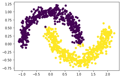
n = 1000, noise = 0.15

# size of data points
n = 1000

# Create the data set
X, y = datasets.make_moons(n_samples = n,
                           noise = 0.15,
                           shuffle = True,
                           random_state=None
                          )
plt.scatter(X[:, 0], X[:, 1])

<matplotlib.collections.PathCollection at 0x7f7a480397f0>

labels = spectral_clustering(X, epsilon)
plt.scatter(X[:, 0], X[:, 1], c = labels)

<matplotlib.collections.PathCollection at 0x7f7a90258310>

From the above plot, we see that our spectral clustering function was able to cluster the dataset successfully when noise = 0.15, n=1000.

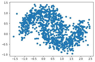
Experiment 3

n = 1000, noise = 0.15

# size of data points
n = 1000

# Create the data set
X, y = datasets.make_moons(n_samples = n,
                           noise = 0.20,
                           shuffle = True,
                           random_state=None
                          )
plt.scatter(X[:, 0], X[:, 1])

<matplotlib.collections.PathCollection at 0x7f7a90277970>

labels = spectral_clustering(X, epsilon)
plt.scatter(X[:, 0], X[:, 1], c = labels)

<matplotlib.collections.PathCollection at 0x7f7a90237d00>

From the above plot - noise = 0.2, n=1000, we see that our spectral clustering function was able to cluster the dataset successfully although the increase of noise makes the area of data points became bigger.

Besides, by comparing the above plots, we found that the distribution of the data points spread more as the noise increased.

Part I

Now try your spectral clustering function on another data set – the bull’s eye!

n = 1000
X, y = datasets.make_circles(n_samples=n, shuffle=True, noise=0.05, random_state=None, factor = 0.4)
plt.scatter(X[:,0], X[:,1])

<matplotlib.collections.PathCollection at 0x7f7a4800e370>

There are two concentric circles. As before k-means will not do well here at all.

km = KMeans(n_clusters = 2)
km.fit(X)
plt.scatter(X[:,0], X[:,1], c = km.predict(X))

<matplotlib.collections.PathCollection at 0x7f7a90775940>

Can your function successfully separate the two circles? Some experimentation here with the value of epsilon is likely to be required. Try values of epsilon between 0 and 1.0 and describe your findings. For roughly what values of epsilon are you able to correctly separate the two rings?

Experiment 1

# Try Epsilon = 0.2
labels = spectral_clustering(X, epsilon = 0.2)
plt.scatter(X[:,0], X[:,1], c = labels)

<matplotlib.collections.PathCollection at 0x7f7a807b5520>

Experiment 2

# Try Epsilon = 0.5
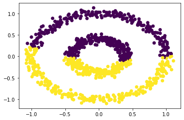
labels = spectral_clustering(X, epsilon = 0.5)
plt.scatter(X[:,0], X[:,1], c = labels)

<matplotlib.collections.PathCollection at 0x7f7a80d9b2b0>

Experiment 3

# Try Epsilon = 0.6
labels = spectral_clustering(X, epsilon = 0.6)
plt.scatter(X[:,0], X[:,1], c = labels)

<matplotlib.collections.PathCollection at 0x7f7a907aefa0>

Experiment 4

# Try Epsilon = 0.8
labels = spectral_clustering(X, epsilon = 0.8)
plt.scatter(X[:,0], X[:,1], c = labels)

<matplotlib.collections.PathCollection at 0x7f7a62f64d30>

​
​

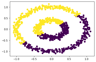
By comparing the above scatter plot, we can see that if the epsilon is less than 0.5 and greater than 0.2, our function cluster the data set succesfully. However, our function can’t successfully cluster the data points if the epsilon is greater than 0.5. In other words, our function cluster the data points well when the epsilon is between (0.2, 0.5)