Blog Post 5 - Image Classification
Distinguishing between cats and dogs might be very easy for everyone! However, this can be a diffcult problem if we want computer to learn to distinguish between them. In this blog plot, we will be learning how to train machine learning models to let our python program to distinguish between cats and dogs. In this blog post, we mainly utilize the packages and methods in TensorFlow.
According to Wikipedia, “TensorFlow is a free and open-source software library for machine learning and artificial intelligence. It can be used across a range of tasks but has a particular focus on training and inference of deep neural networks.”
Note: Some part of code chunks in this blog post are provided by Professor Phil Chodrow in PIC16B course at UCLA. Some part of code chunks and methods are based on TensorFlow Tutorial Page.
§1. Import and Obtain Data
First of all, we need to import some necessary packages!
import os
import tensorflow as tf
from tensorflow.keras import utils
import matplotlib.pyplot as plt
import random
import numpy as np
from tensorflow.keras import layers
from tensorflow.keras import models
Now, let’s access the dataset. We’ll use a sample data set provided by the TensorFlow team that contains labeled images of cats and dogs.
Now, let’s run the following code block and see what is going to happen!
# location of data
_URL = 'https://storage.googleapis.com/mledu-datasets/cats_and_dogs_filtered.zip'

# download the data and extract it
path_to_zip = utils.get_file('cats_and_dogs.zip', origin=_URL, extract=True)

# construct paths
PATH = os.path.join(os.path.dirname(path_to_zip), 'cats_and_dogs_filtered')

train_dir = os.path.join(PATH, 'train')
validation_dir = os.path.join(PATH, 'validation')

# parameters for datasets
BATCH_SIZE = 32
IMG_SIZE = (160, 160)

# construct train and validation datasets
train_dataset = utils.image_dataset_from_directory(train_dir,
                                                   shuffle=True,
                                                   batch_size=BATCH_SIZE,
                                                   image_size=IMG_SIZE)

validation_dataset = utils.image_dataset_from_directory(validation_dir,
                                                        shuffle=True,
                                                        batch_size=BATCH_SIZE,
                                                        image_size=IMG_SIZE)

# construct the test dataset by taking every 5th observation out of the validation dataset
val_batches = tf.data.experimental.cardinality(validation_dataset)
test_dataset = validation_dataset.take(val_batches // 5)
validation_dataset = validation_dataset.skip(val_batches // 5)

# Extract the class_names, we will use this later
class_names = train_dataset.class_names
Found 2000 files belonging to 2 classes.
Found 1000 files belonging to 2 classes.
After running the above code blocks, we successfully obtained the TensorFlow Dataset for our training, validation, and testing tasks. In this case, we used a special-purpose keras utility named image_dataset_from_directory to construct a Dataset. The shuffle argument above means that the order of the retrieved data from the directory will be randomized. The batch_size determines how many data points will be obtained from the directory at each time. In our example, we can see that each request we made will get 32 images from each of the data sets. Lastly, the iamge_size argument will specifies the size of the input images.
The following code can help us rapidly read the data. We just need to paste it and run it. If you are interested in learning more about this code, feel free to take a look at this web page
AUTOTUNE = tf.data.AUTOTUNE

train_dataset = train_dataset.prefetch(buffer_size=AUTOTUNE)
validation_dataset = validation_dataset.prefetch(buffer_size=AUTOTUNE)
test_dataset = test_dataset.prefetch(buffer_size=AUTOTUNE)
Working with Datasets
If we want to get a piece of data set, we can definitely use take method. For example, train_dataset.take(1) will retrieve 32 images with labels from our training data.
In order to further explore our cute cats and dogs data set, we are going to write a function to create a two-row, three column visualization. In the first row of our visualization, we want to show three random pictures of cats. In the second rows of our visualization, we want to show three random pictures of dogs. We may take a look at some related code in the TensorFlow tutorial.
def visualize_img():
    '''
    This function generate a
    two-row, three-column visualization of
    the random pictures of cats and dogs
    '''
    # Set the figure size
    plt.figure(figsize=(12, 8))

    # Initialize a list of cats and dogs
    cats_image, dogs_image = [], []
    # Write a for loop to take a batch of images
    for images, labels in train_dataset.take(1):
        # seperate the images of cats and dogs
        # in two different lists.
        for i in range(0, len(labels)):
            if class_names[labels[i]] == "cats":
                cats_image.append(i)
            else:
                dogs_image.append(i)

    # Randomly select 3 cats and 3 dogs
    three_random_cats = random.sample(cats_image, 3)
    three_random_dogs = random.sample(dogs_image, 3)

    # Merging two lists together
    cats_and_dogs = three_random_cats + three_random_dogs

    # Initialize count number for cats and dogs
    count_cats = 1
    count_dogs = 1

    # draw the first three plots of cats
    for i in cats_and_dogs:
        # determine whether it is a cat or dog,
        # if it is a cat draw the visualization on first row.
        if class_names[labels[i]] == "cats":
            if count_cats < 4:
                ax1 = plt.subplot(2, 3, count_cats)
                plt.imshow(images[i].numpy().astype("uint8"))
                plt.axis("off")
                plt.title(class_names[labels[i]])
                count_cats = count_cats + 1
             else:
                continue
      # Draw next three plots of dogs
    for j in cats_and_dogs:
        # Determine whether it is a dog,
        # if it is a dog, draw the visualization on the second row.
        if class_names[labels[j]] == "dogs":
            if count_dogs < 4:
                ax1 = plt.subplot(2, 3, count_dogs+3)
                plt.imshow(images[j].numpy().astype("uint8"))
                plt.axis("off")
                plt.title(class_names[labels[j]])
                count_dogs = count_dogs + 1
            else:
                continue
visualize_img()
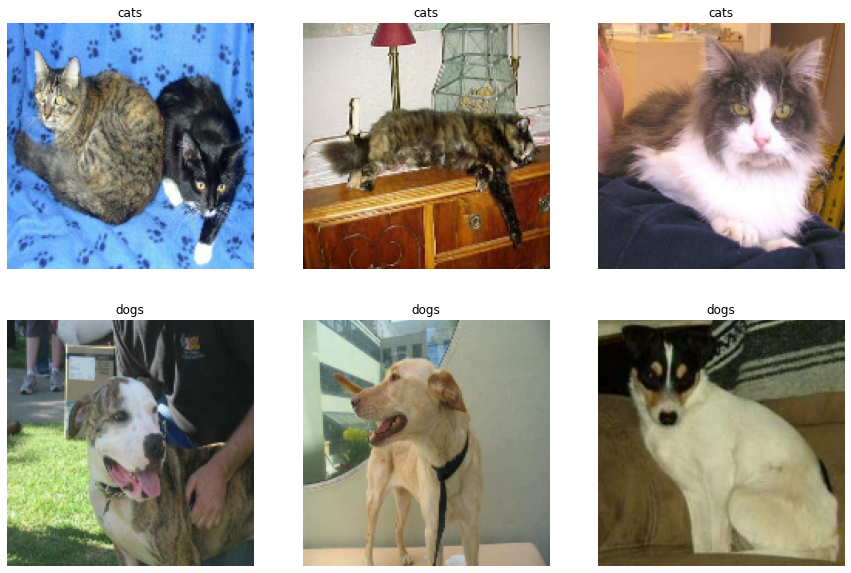
Looks great! The first row shows three images of cats, and the second row shows three images of dogs!
Check Label Frequencies
Compute the number of images in the training data with label 0 (corresponding to “cat”) and label 1 (corresponding to “dog”). A baseline machine learning is a model that always guesses the most frequent label. In our case, we have a total 2000 images, let’s go ahead and compute the accuracy of our baseline machine learning model!
The following line of code will create an iterator called labels.
labels_iterator = train_dataset.unbatch().map(lambda image, label: label).as_numpy_iterator()
sum(labels_iterator)
1000
baseline = 1000 / 2000
baseline
0.5
In our case, the baseline accuracy of the model is 0.5!
§2. First Model
Now, we are going to create our first model! A tf.keras.Sequential model. In our model, we should include at least two Conv2D layers, at least two MaxPooling2D layers, at least one Flatten layer, at least one Dense layer, and at least one Dropout layer. Our first model will initalize 2000 images without using any data augmentation and preprocessing. Our goal for this model is to achieve 52% validation accuracy. Let’s create and fit our model to see the accuracy of this model, and whether it is overfitting.
Model 1
model1 = models.Sequential([
    layers.Conv2D(32, (3, 3), activation='relu',input_shape=(160,160,3)),
    layers.MaxPooling2D((2, 2)),

    layers.Conv2D(32, (3, 3), activation='relu'),
    layers.Conv2D(32, (3, 3), activation='relu'),
    layers.MaxPooling2D((2, 2)),

    layers.Conv2D(32, (3, 3), activation='relu'),
    layers.Conv2D(32, (3, 3), activation='relu'),
    layers.MaxPooling2D((2, 2)),

    layers.Flatten(),
    # Large number for dense can improve our model
    layers.Dense(2048, activation='relu'),
    # Dropout can improve the overfitting.
    layers.Dropout(0.5),
    layers.Dense(2)
])
model1.summary()
Model: "sequential"
_________________________________________________________________
 Layer (type)                Output Shape              Param #
=================================================================
 conv2d (Conv2D)             (None, 158, 158, 32)      896

 max_pooling2d (MaxPooling2D  (None, 79, 79, 32)       0
 )

 conv2d_1 (Conv2D)           (None, 77, 77, 32)        9248

 conv2d_2 (Conv2D)           (None, 75, 75, 32)        9248

 max_pooling2d_1 (MaxPooling  (None, 37, 37, 32)       0
 2D)

 conv2d_3 (Conv2D)           (None, 35, 35, 32)        9248

 conv2d_4 (Conv2D)           (None, 33, 33, 32)        9248

 max_pooling2d_2 (MaxPooling  (None, 16, 16, 32)       0
 2D)

 flatten (Flatten)           (None, 8192)              0

 dense (Dense)               (None, 2048)              16779264

 dropout (Dropout)           (None, 2048)              0

 dense_1 (Dense)             (None, 2)                 4098

=================================================================
Total params: 16,821,250
Trainable params: 16,821,250
Non-trainable params: 0
_________________________________________________________________
model1.compile(optimizer='adam',
               loss=tf.keras.losses.SparseCategoricalCrossentropy(from_logits=True),
               metrics=['accuracy'])

history = model1.fit(train_dataset,
                     epochs=20,
                     validation_data=validation_dataset)
plt.figure(figsize=(8,6))
plt.plot(history.history["accuracy"], label = "Training")
plt.plot(history.history["val_accuracy"], label = "Validation")
plt.axhline(y=0.50, color="black", label = "Baseline 50%")
plt.gca().set(xlabel = "epoch", ylabel = "Accuracy")
plt.ylim([0,1.1])
plt.legend()
<matplotlib.legend.Legend at 0x7f6a6239b950>
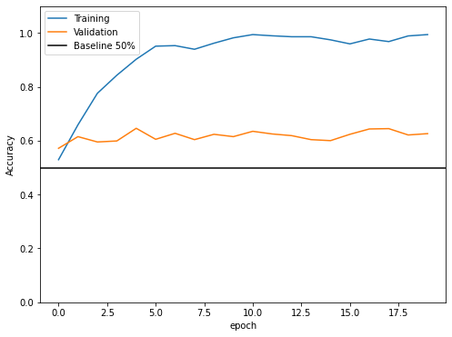
The validation accuracy of my model stabilized between 57% and 64%.
In this model, we reached the highest validation accuracy of 64%, and our training accuracy reached 99%. Compare to the baseline, we achieve around 10-14% better than the 50% baseline. However, it is obviously there exists overfitting in our model because the training accuracy is much higher than the validation accuracy.
§3. Model with Data Augmentation
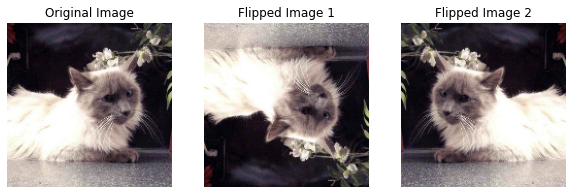
Now, we are going to add some data augmentation layers to our model to see if we can improve our model accuracy. When a picture of a cat or dog is filpped, they are still dogs/cats. In order to improve our model, we can include such trainformed version of the image in our training process. First, let’s try to create some visualization to see how it works.
Visualize Random Flip & Random Rotation
The follow code flipped the image of a cat in either horizontal and vertical way.
data_flip = tf.keras.Sequential([
    tf.keras.layers.RandomFlip("horizontal_and_vertical")
])

plt.figure(figsize=(10, 10))
for images, labels in train_dataset.take(1):
    one_image = images[0]


for i in range(0, 3):
    if i == 0:
        ax = plt.subplot(2, 3, 1)
        plt.imshow(one_image / 255)
        plt.title("Original Image")
        plt.axis("off")
    else:
        ax = plt.subplot(2, 3, i+1)
        flip_img = data_flip(one_image)
        plt.imshow(flip_img / 255)
        plt.title("Flipped Image " + str(i))
        plt.axis("off")
The following code rotated a picture of a dog with 20% degree.
data_rotate = tf.keras.Sequential([
    tf.keras.layers.RandomRotation(0.2)
])
plt.figure(figsize=(12, 10))
for images, labels in train_dataset.take(1):
    one_image = images[0]

for i in range(0, 3):
    if i == 0:
        ax = plt.subplot(2, 3, 1)
        plt.imshow(one_image / 255)
        plt.title("Original Image")
        plt.axis("off")
    else:
        ax = plt.subplot(2, 3, i+1)
        rotate_img = data_rotate(one_image)
        plt.imshow(rotate_img / 255)
        plt.title("Flipped Image " + str(i))
        plt.axis("off")

Model 2
Now, let’s create our new tf.keras.models.Sequential model called model2. We should put our augmentation layers in the first two layers. We will use both RandomFlip() layers and RandomRotation() layers. Our goal in this second model is to reach at least 55% validation accuracy. Let’s go ahead and fit our model!
model2 = models.Sequential([
    layers.InputLayer(input_shape=(160, 160, 3)),
    tf.keras.layers.RandomFlip("horizontal_and_vertical"),
    tf.keras.layers.RandomRotation(0.25),

    layers.Conv2D(32, (3, 3), activation='relu', input_shape=(160, 160, 3)),
    layers.Conv2D(32, (3, 3), activation='relu'),
    layers.MaxPooling2D((2, 2)),

    layers.Conv2D(32, (3, 3), activation='relu'),
    layers.Conv2D(32, (3, 3), activation='relu'),
    layers.MaxPooling2D((2, 2)),

    layers.Conv2D(32, (3, 3), activation='relu'),
    layers.Conv2D(32, (3, 3), activation='relu'),
    layers.MaxPooling2D((2, 2)),

    layers.Flatten(),
    # Large number for dense can improve our model
    layers.Dense(2048, activation='relu'),
	# Use Dropout to improve overfitting
    layers.Dropout(0.5),
    layers.Dense(1, activation="sigmoid")
])
model2.summary()
Model: "sequential_21"
_________________________________________________________________
 Layer (type)                Output Shape              Param #
=================================================================
 random_flip_15 (RandomFlip)  (None, 160, 160, 3)      0

 random_rotation_18 (RandomR  (None, 160, 160, 3)      0
 otation)

 conv2d_69 (Conv2D)          (None, 158, 158, 32)      896

 conv2d_70 (Conv2D)          (None, 156, 156, 32)      9248

 max_pooling2d_63 (MaxPoolin  (None, 78, 78, 32)       0
 g2D)

 conv2d_71 (Conv2D)          (None, 76, 76, 32)        9248

 conv2d_72 (Conv2D)          (None, 74, 74, 32)        9248

 max_pooling2d_64 (MaxPoolin  (None, 37, 37, 32)       0
 g2D)

 conv2d_73 (Conv2D)          (None, 35, 35, 32)        9248

 conv2d_74 (Conv2D)          (None, 33, 33, 32)        9248

 max_pooling2d_65 (MaxPoolin  (None, 16, 16, 32)       0
 g2D)

 flatten_12 (Flatten)        (None, 8192)              0

 dense_24 (Dense)            (None, 2048)              16779264

 dropout_12 (Dropout)        (None, 2048)              0

 dense_25 (Dense)            (None, 1)                 2049

=================================================================
Total params: 16,828,449
Trainable params: 16,828,449
Non-trainable params: 0
_________________________________________________________________
model2.compile(optimizer = "adam",
               loss=tf.keras.losses.BinaryCrossentropy(),
               metrics=['accuracy'])

history2 = model2.fit(train_dataset,
                     epochs=20,
                     validation_data=validation_dataset)
plt.figure(figsize=(8,6))
plt.plot(history2.history["accuracy"], label = "Training")
plt.plot(history2.history["val_accuracy"], label = "Validation")
plt.axhline(y=0.55, color="green", label = "55% Line")
plt.gca().set(xlabel = "epoch", ylabel = "Accuracy")
plt.ylim([0,1.1])
plt.legend()
<matplotlib.legend.Legend at 0x7f805ae1b4d0>
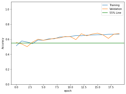
In model2, we reached the highest validation accuracy of 67%, and 66.8% training accuracy.
Compare to the validation accuracy we obtained from model1, model2 is 5% higher. The issues of overfitting has been improved compared to model 1. Although at some Epochs we might observe a little bit overfitting, the training accuracy and the validation accuracy is getting closer at each training Epochs.
§4. Data Preprocessing
It is helpful to make some simple transformations to the input data sometimes. In this part, we are going to do some data preprocessing to see if it can improve our model accuracy! For example, many models can train faster with RGB values normalized between 0 and 1 rather than between 0 and 255. By doing this way, we can pend more of our training energy handling actual signal in the data and less energy having the weights adjust to the data scale.
Model 3
The following code will create a preprocessing layer called preprocessor which you can slot into your model pipeline.
i = tf.keras.Input(shape=(160, 160, 3))
x = tf.keras.applications.mobilenet_v2.preprocess_input(i)
preprocessor = tf.keras.Model(inputs = [i], outputs = [x])
Now, let’s create our model3! It is recommended that we can put the preprocessor layer at the very first layer before our data augmentation layers.
model3 = models.Sequential([

    preprocessor,

    tf.keras.layers.RandomFlip("horizontal"),
    tf.keras.layers.RandomRotation(0.25),

    layers.Conv2D(32, (3, 3), activation='relu'),
    layers.MaxPooling2D((2, 2)),

    layers.Conv2D(32, (3, 3), activation='relu'),
    layers.MaxPooling2D((2, 2)),

    layers.Conv2D(32, (3, 3), activation='relu'),
    layers.MaxPooling2D((2, 2)),

    layers.Flatten(),
    # Large number for dense can improve our model
    layers.Dense(2048, activation='relu'),
	# Dropout can improve overfitting
    layers.Dropout(0.75),
    layers.Dense(1, activation="sigmoid")

])

model3.compile(optimizer = "adam",
               loss=tf.keras.losses.BinaryCrossentropy(),
               metrics=['accuracy'])

history3 = model3.fit(train_dataset,
                     epochs=20,
                     validation_data=validation_dataset)
model3.summary()
Model: "sequential_23"
_________________________________________________________________
 Layer (type)                Output Shape              Param #
=================================================================
 model_3 (Functional)        (None, 160, 160, 3)       0

 random_flip_17 (RandomFlip)  (None, 160, 160, 3)      0

 random_rotation_20 (RandomR  (None, 160, 160, 3)      0
 otation)

 conv2d_75 (Conv2D)          (None, 158, 158, 32)      896

 max_pooling2d_66 (MaxPoolin  (None, 79, 79, 32)       0
 g2D)

 conv2d_76 (Conv2D)          (None, 77, 77, 32)        9248

 max_pooling2d_67 (MaxPoolin  (None, 38, 38, 32)       0
 g2D)

 conv2d_77 (Conv2D)          (None, 36, 36, 32)        9248

 max_pooling2d_68 (MaxPoolin  (None, 18, 18, 32)       0
 g2D)

 flatten_13 (Flatten)        (None, 10368)             0

 dense_27 (Dense)            (None, 2048)              21235712

 dropout_14 (Dropout)        (None, 2048)              0

 dense_28 (Dense)            (None, 1)                 2049

=================================================================
Total params: 21,257,153
Trainable params: 21,257,153
Non-trainable params: 0
_________________________________________________________________
plt.figure(figsize=(8,6))
plt.plot(history3.history["accuracy"], label = "Training")
plt.plot(history3.history["val_accuracy"], label = "Validation")
plt.axhline(y=0.70, color="green", label = "70% Line")
plt.gca().set(xlabel = "epoch", ylabel = "Accuracy")
plt.ylim([0,1.1])
plt.legend()
<matplotlib.legend.Legend at 0x7f805b104f90>
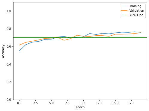
The validation accuracy of model 3 reached the highest accuracy of 75% with 75.8% training accuracy.
The validation accuracy of model3 reached a higher score compared to model2. The issue of overfitting was also improved. The training accuracy is closer to validation accuracy at each Epoch.
§5. Transfer Learning
So far, we’ve trained three differnt models. As we add augumentation and transformation, our model is getting better. However, someone may have already trained a model that does a similar task. Let’s try if we can use a pre-existing model for our case!
We will have to first access this pre-existing base model Let’s paste the following code to download MobileNetV2 and make it as a layer to be included in our model! Our goal for this taks is to reach at least 95% validation accuracy.
IMG_SHAPE = IMG_SIZE + (3,)
base_model = tf.keras.applications.MobileNetV2(input_shape=IMG_SHAPE,
                                               include_top=False,
                                               weights='imagenet')
base_model.trainable = False

i = tf.keras.Input(shape=IMG_SHAPE)
x = base_model(i, training = False)
base_model_layer = tf.keras.Model(inputs = [i], outputs = [x])
In order to create our model4 using MobileNetV2, we will have to use the following layers:
-
The
preprocessorlayer from Part §4. -
The data augmentation layers from Part §3.
-
The
base_model_layerconstructed above. -
A
Dense(2)layer at the very end to actually perform the classification.
Since Dense(2) doesn’t work on my Google Colab, I’ve changed to use Dense(1).
model4 = models.Sequential([
    preprocessor,

    layers.RandomFlip("horizontal_and_vertical"),
    layers.RandomRotation(0.2),

    base_model_layer,
    layers.GlobalAveragePooling2D(),
    # Use Dropout to improve the model
    layers.Dropout(0.4),
    layers.Dense(1, activation="sigmoid")
])

model4.compile(optimizer = "adam",
               loss=tf.keras.losses.BinaryCrossentropy(),
               metrics=['accuracy'])

history4 = model4.fit(train_dataset,
                     epochs=20,
                     validation_data=validation_dataset)
model4.summary()
Model: "sequential_22"
_________________________________________________________________
 Layer (type)                Output Shape              Param #
=================================================================
 model_1 (Functional)        (None, 160, 160, 3)       0

 random_flip_16 (RandomFlip)  (None, 160, 160, 3)      0

 random_rotation_19 (RandomR  (None, 160, 160, 3)      0
 otation)

 model_2 (Functional)        (None, 5, 5, 1280)        2257984

 global_average_pooling2d (G  (None, 1280)             0
 lobalAveragePooling2D)

 dropout_13 (Dropout)        (None, 1280)              0

 dense_26 (Dense)            (None, 1)                 1281

=================================================================
Total params: 2,259,265
Trainable params: 1,281
Non-trainable params: 2,257,984
_________________________________________________________________
plt.figure(figsize=(8,6))
plt.plot(history4.history["accuracy"], label = "Training")
plt.plot(history4.history["val_accuracy"], label = "Validation")
plt.axhline(y=0.95, color="green", label = "95% Line")
plt.gca().set(xlabel = "epoch", ylabel = "Accuracy")
plt.ylim([0,1.1])
plt.legend()
<matplotlib.legend.Legend at 0x7f805aa17c10>

Wow, as we can see from the above visualization, the validation accuracy reached the highest score of 97%, and the training accuracy reached 92%.
Compare to last part, we did almost 20% better in validation accuracy and training accuracy. However, it might exists a little bit overfitting in our model.
§6. Score on Test Data
Eventually, let’s evaluate the valication accuracy of our most performant model! on the unseen test_dataset. Based on the above model1 to model4, it is obvious that model4 is our best model!
model4.evaluate(test_dataset)
6/6 [==============================] - 0s 25ms/step - loss: 0.0552 - accuracy: 0.9896


[0.05519675835967064, 0.9895833134651184]
From the above output, we can see that the accuracy is about 98.9% which is awesome comparing to our first model! This means that this model can distinguish between cats and dogs with at least 98.9% accuracy. It also shows that using MobileNetV2 can make a better model. However, this method would take a little bit longer to train the dataset. We can also see from model4.summary(), the model is much more complex than other models.