Blog Post 6 - Fake News Classification Using TensorFlow
With the development of the Internet, the news media has become faster and faster to spread. However, some fake news reports have also appeared in the Internet along with it. Some fake news media hope to arouse public opinion through fake news, so as to increase their own influence in the internet. Hence, it is important for everyone to have the ability to recognize the real and fake news.
In this blog post, we are going to develop a fake news classifier using Tensorflow from Python. It is highly recommended to work on this blog post in Google Colab.
Data Source
Our data for this blog post comes from the following source:
- Ahmed H, Traore I, Saad S. (2017) “Detection of Online Fake News Using N-Gram Analysis and Machine Learning Techniques. In: Traore I., Woungang I., Awad A. (eds) Intelligent, Secure, and Dependable Systems in Distributed and Cloud Environments. ISDDC 2017. Lecture Notes in Computer Science, vol 10618. Springer, Cham (pp. 127-138).
We can access it from Kaggle. The data has been done a small amount of data cleaning, and performed a train-test split by Professor Phil Chodrow.
Now, let’s get start!
§1. Acquire Training Data
The following URL is the training data set. We can either read it into our Jupyter Notebook directly or download it to our computer and read it from disk. In this blog, we will use pd.read_csv() to read it into Python directly.
train_url = "https://github.com/PhilChodrow/PIC16b/blob/master/datasets/fake_news_train.csv?raw=true"
Before we read the data, we need to import required packages.
import pandas as pd
import numpy as np
import tensorflow as tf
import string
import re
# Read the data set
df = pd.read_csv(train_url)
# Let's take a quick look
df.head()
| Unnamed: 0 | title | text | fake | |
|---|---|---|---|---|
| 0 | 17366 | Merkel: Strong result for Austria's FPO 'big c... | German Chancellor Angela Merkel said on Monday... | 0 |
| 1 | 5634 | Trump says Pence will lead voter fraud panel | WEST PALM BEACH, Fla.President Donald Trump sa... | 0 |
| 2 | 17487 | JUST IN: SUSPECTED LEAKER and “Close Confidant... | On December 5, 2017, Circa s Sara Carter warne... | 1 |
| 3 | 12217 | Thyssenkrupp has offered help to Argentina ove... | Germany s Thyssenkrupp, has offered assistance... | 0 |
| 4 | 5535 | Trump say appeals court decision on travel ban... | President Donald Trump on Thursday called the ... | 0 |
From the above pandas dataframe, we can see that each row of the data corresponds to an news article. The title column is the title of the article, and the text column is the full article text. The last column fake is 0 if the article is true and 1 if the article contains fake news.
§2. Make a Dataset
Now, we are going to write a function call make_dataset. This function will do following two things:
-
Remove the stopwords from the article
textandtitle. Note that a stopword means a word that is usually considered to be uninformative. For exampl, stopwords could be: “the”, “but”, “and”, “or”. We can get help from this StackOverFlow thread. -
Our function should construct and return a
tf.data.Dataset, and the function should contains two inputs and one output. Input should be of the form(title, text). The output should only contains thefakecolumn.
Write The Function
First, we import stopwords from nltk.corpus
# Import stopwords
import nltk
from nltk.corpus import stopwords
# Download stopwords
nltk.download('stopwords')
# Extract stopwords
stop = stopwords.words('english')
[nltk_data] Downloading package stopwords to /root/nltk_data...
[nltk_data] Package stopwords is already up-to-date!
def make_dataset(df):
# remove stopwords from texts and articles
df['text_without_stop'] = df['text'].apply(lambda x: ' '.join([word for word in x.split() if word not in (stop)]))
df['title_without_stop'] = df['title'].apply(lambda x: ' '.join([word for word in x.split() if word not in (stop)]))
# contruct the dataset
data = tf.data.Dataset.from_tensor_slices(
(
{
"title" : df[["title_without_stop"]],
"text" : df[["text_without_stop"]]
},
{
"fake" : df[["fake"]]
}
)
)
# we shuffle the dataset
data = data.shuffle(buffer_size = len(data))
# batch our dataset to increase the training speed
data = data.batch(100)
return data
Next, we call our function make_dataset() on our training dataframe to produce a Dataset. I’ve included data = data.batch(100) prior to returning our dataset. Batching causes our model to train on chunks of data rather than individual rows. Although sometimes batching can reducen the accuracy, but it can also increase the speed of training. It is important to find a balance. I found that batches of 100 rows worked well.
data = make_dataset(df)
Validation Data
After we have constucted our primary Dataset, we split 20% of it to use for validation.
train_size = int(0.8*len(data))
val_size = int(0.2*len(data))
train_dataset = data.take(train_size)
val_dataset = data.take(val_size)
# Checking the size of training and validation set
len(train_dataset), len(val_dataset)
(180, 45)
Base Rate
We know that the base rate refers to the accuracy of a model that always makes the same guess. Now, we need to determine the base rate for this data set by checking the labels on our training data set.
a = list(data.as_numpy_iterator())[0]
labels = a[1].values()
print(sum(list(labels)[0] == 0))
print(sum(list(labels)[0] == 1))
# Compute the Base Rate
47 / 100
[44]
[56]
0.47
We can see that the base rate is 47%, which is close to the 50%.
§3. Create Models
Now, we are going to create our TensorFlow model to give a perspective for the following question:
When detecting fake news, is it most effective to focus on only the title of the article, the full text of the article, or both?
In order to answer the above question, we will create three TensorFlow models.
-
First model, we use only the article title as input.
-
Second model, we use only the article text as input.
-
Third model, we use both the article title and the article text as input.
Let’s train our model until they appear to be fully trained. And we will compare their performance! We will need to use the Function API, rather than the Sequential API for this modeling task.
Standardization and Vectorization
First, we want to convert all text to lowercase and remove punctuation. Then, we want to vectorize the text by representing text as a vector (array, tensor).
# Import necessary packages
import string
import re
from tensorflow.keras.layers.experimental.preprocessing import TextVectorization
from tensorflow.keras import Input, layers, Model, utils, losses
# set size_vocabulary equal to 2000
size_vocabulary = 2000
# define standardization function
def standardization(input_data):
lowercase = tf.strings.lower(input_data)
no_punctuation = tf.strings.regex_replace(lowercase,
'[%s]' % re.escape(string.punctuation),'')
return no_punctuation
# set vectorize layer
vectorize_layer = TextVectorization(
standardize=standardization,
max_tokens=size_vocabulary, # only consider this many words
output_mode='int',
output_sequence_length=500)
# vectorize both title and text
vectorize_layer.adapt(train_dataset.map(lambda x, y: x["title"]))
vectorize_layer.adapt(train_dataset.map(lambda x, y: x["text"]))
Construct Model
Now, we’ve successfully prepared our data, and it’s time to construct our models! The first step is to specifiy the two kinds of keras.Input for our model.
# specify input for title
title_input = Input(
shape = (1,),
name = "title",
dtype = "string"
)
# specify input for text
text_input = Input(
shape = (1,),
name = "text",
dtype = "string"
)
Hidden Layers
Now, we are going to write a pipeline for the titles and text. Since title and text are different part of text but share similar vocabulary, we are going to use shared layers for input.
# Use sharing embedding
embedding = layers.Embedding(size_vocabulary, 16, name = "embedding")
# First, we write a pipeline for the title
title_features = vectorize_layer(title_input)
title_features = embedding(title_features)
title_features = layers.Dropout(0.2)(title_features)
title_features = layers.GlobalAveragePooling1D()(title_features)
title_features = layers.Dropout(0.2)(title_features)
title_features = layers.Dense(32, activation='relu')(title_features)
# Next, we write a pipeline for the text
text_features = vectorize_layer(text_input)
text_features = embedding(text_features)
# Here I increased the dropout to 0.75 to avoid
# large overfitting when training model2
text_features = layers.Dropout(0.75)(text_features)
text_features = layers.GlobalAveragePooling1D()(text_features)
text_features = layers.Dropout(0.5)(text_features)
text_features = layers.Dense(32, activation='relu')(text_features)
# output layers for model 1
title_output = layers.Dense(2, name = "fake")(title_features)
# output layers for model 2
text_output = layers.Dense(2, name = "fake")(text_features)
# output layers for model 3
main = layers.concatenate([title_features, text_features], axis = 1)
main = layers.Dense(32, activation='relu')(main)
model3_output = layers.Dense(2, name = "fake")(main)
Now, it’s time to create our model! In order to save our time, I’ve enclose the model training process in a function called training_model. We are able to re-use this function for our model1, model2, and model3.
from matplotlib import pyplot as plt
# enclosed training process in a function to
# repeatedly use in model 1,2,3
def training_model(input, output):
# create model
model = Model(
inputs = input,
outputs = output
)
# Complile the model
model.compile(optimizer = "adam",
loss = losses.SparseCategoricalCrossentropy(from_logits=True),
metrics=['accuracy']
)
# train the model
history = model.fit(train_dataset,
validation_data=val_dataset,
epochs = 50,
verbose = False)
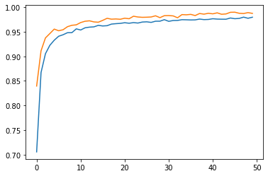
# plot the training and validation accuracy
plt.plot(history.history["accuracy"])
plt.plot(history.history["val_accuracy"])
# return result
return model, history
Model 1: Train Using Title
model1, history1 = training_model(title_input, title_output)
/usr/local/lib/python3.7/dist-packages/keras/engine/functional.py:559: UserWarning: Input dict contained keys ['text'] which did not match any model input. They will be ignored by the model.
inputs = self._flatten_to_reference_inputs(inputs)

# Visualiza the structure of our model1
tf.keras.utils.plot_model(model1)
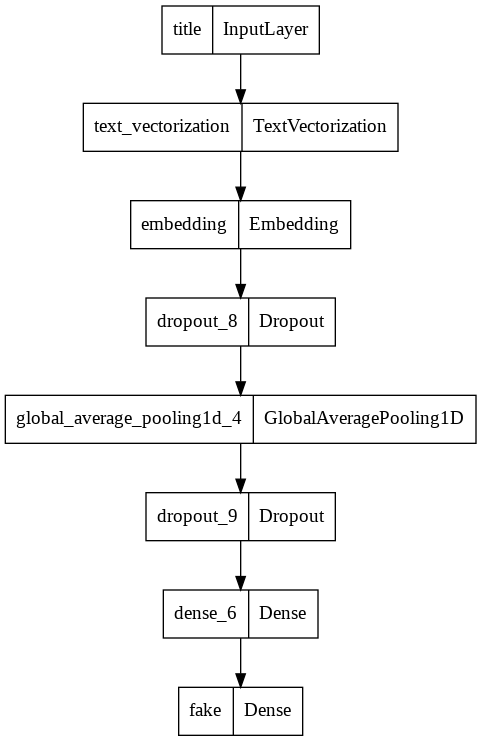
# Output the maximum validation accuracy of model1
round(max(history1.history["val_accuracy"]),5)
0.98978
From the above result, we can see that our the validation accuracy of our model 1 reached around 98.978%, which is not bad! However, we can do it better in our next model!
Model 2: Train Using Text
model2, history2 = training_model(text_input, text_output)
/usr/local/lib/python3.7/dist-packages/keras/engine/functional.py:559: UserWarning: Input dict contained keys ['title'] which did not match any model input. They will be ignored by the model.
inputs = self._flatten_to_reference_inputs(inputs)
# Visualiza the structure of our model2
tf.keras.utils.plot_model(model2)
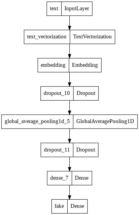
# Output the maximum validation accuracy of model2
round(max(history2.history["val_accuracy"]),5)
0.99
Our model2 reached 99% validation accuracy, which is better than model1! Let’s now move to model 3 and see if the accuracy can still be improved!
Model 3
model3, history3 = training_model([title_input, text_input], model3_output)

# Visualiza the structure of our model3
tf.keras.utils.plot_model(model3)
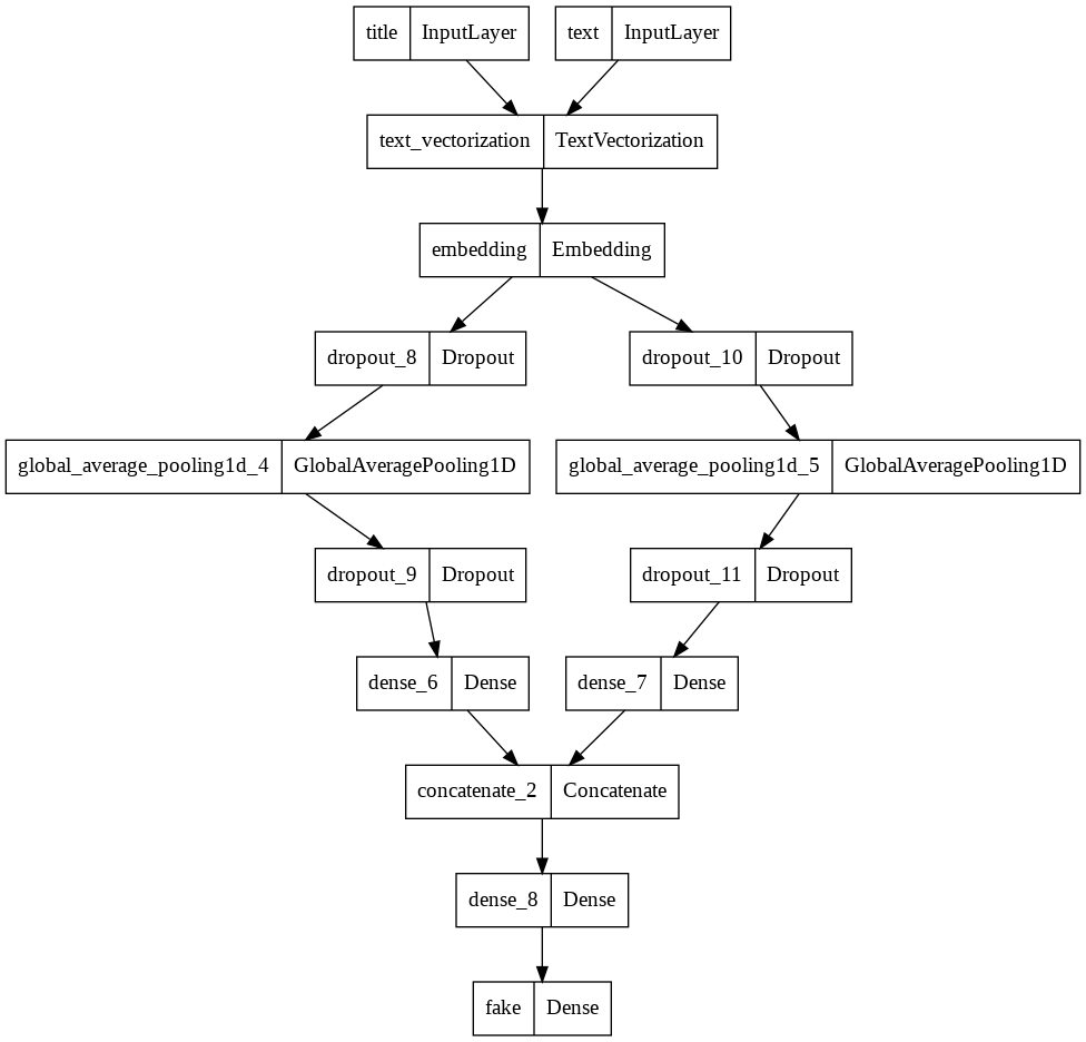
# Output the maximum validation accuracy of model3
round(max(history3.history["val_accuracy"]))
1
By comparing the above model1, model2, model3, we conclude that model3 is the best model because this model is able to consistently obtain at least 99% accuracy on the validation set. And the best validation set reached the highest score of 100%!
§4. Model Evaluation
In this part, we are going to test our model performance on unseen test data set. We will focus on our best model: Model 3 and ignore model1 and model2.
Now, we first download the test data from the following URL:
test_url = "https://github.com/PhilChodrow/PIC16b/blob/master/datasets/fake_news_test.csv?raw=true"
We would have to convert this test data using the make_dataset function we have created in Part 2. Then, we evaluate our best model on this data.
test_data = pd.read_csv(test_url)
test_dataset = make_dataset(test_data)
Then, we evaluate the data
model3.evaluate(test_dataset)
225/225 [==============================] - 2s 9ms/step - loss: 0.0195 - accuracy: 0.9950
[0.019546041265130043, 0.9949663877487183]
According to the above result, we can see that we are able to correctly detect and classify a fake news with 99.5% accuracy.
§5. Embedding Visualization
In this last section, we are going to take a look at the embedding learned by our model!
# get the weights from the embedding layer
weights = model3.get_layer('embedding').get_weights()[0]
# get the vocabulary from our data prep for later
vocab = vectorize_layer.get_vocabulary()
# import PCA
from sklearn.decomposition import PCA
pca = PCA(n_components=2)
weights = pca.fit_transform(weights)
embedding_df = pd.DataFrame({
'word' : vocab,
'x0' : weights[:,0],
'x1' : weights[:,1]
})
import plotly.express as px
fig = px.scatter(embedding_df,
x = "x0",
y = "x1",
size = list(np.ones(len(embedding_df))),
size_max = 5,
hover_name = "word")
# show the figure
fig.show()
Everything looks great! We’ve successfully visualize our embedding. From the above visualization, we found that some points of words are far away from the center of the plot. For example, trump, obamas, myanmar, rohingya, reportedly, gop.
Whenever we create a machine learning model, it is our responsibility to understand the limitations and biases of our model. Now, let’s find out what kinds of words in our model associates with democrat and republican.
democrat = ['democrat']
republican = ['republican']
highlight_1 = ["liberal", "biden", "left", "equality"]
highlight_2 = ["trumps", "fake", "conservative", "energy"]
def mapper(x):
if x in democrat:
return 1
elif x in republican:
return 4
elif x in highlight_1:
return 3
elif x in highlight_2:
return 2
else:
return 0
embedding_df["highlight"] = embedding_df["word"].apply(mapper)
embedding_df["size"] = np.array(1.0 + 50*(embedding_df["highlight"] > 0))
fig2 = px.scatter(embedding_df,
x = "x0",
y = "x1",
color = "highlight",
size = list(embedding_df["size"]),
size_max = 20,
hover_name = "word")
fig2.show()
By observing the above plot, we found that:
-
word
Republicanis far away from the wordliberal. -
word
trumpis far away from the center of the plot. -
word
democratis more close to the center of the plot. -
word
bidenis more close toenergy
The reason we observed these is that: for example, Biden always pay attention to the new energy during his presidency. Republican and democrat represent two different parties in the United States, and they would probably have different thoughts on different topics.